Manual Mode

The manual mode of OpihiExarata is its asteroid view-finding mode. Although, photometric monitoring can be done manually, and the manual mode is well equipped for said use case, it is not the primary use case for the manual mode.

The user uses the Opihi instrument to take images of an asteroid. Then they specify the location of the asteroid using a GUI (usually with help from comparing their image to a reference image). An astrometric solution can convert the asteroid’s pixel location to an on-sky location. Then by utilizing previous observations, its path across the sky can be determined. This information is used to properly point the IRTF telescope to the desired asteroid target.

We present the procedure for operating OpihiExarata in its manual mode, please also reference the GUI figure provided for reference. We also summarize the procedure and process of the manual mode via a flowchart.

Graphical User Interface

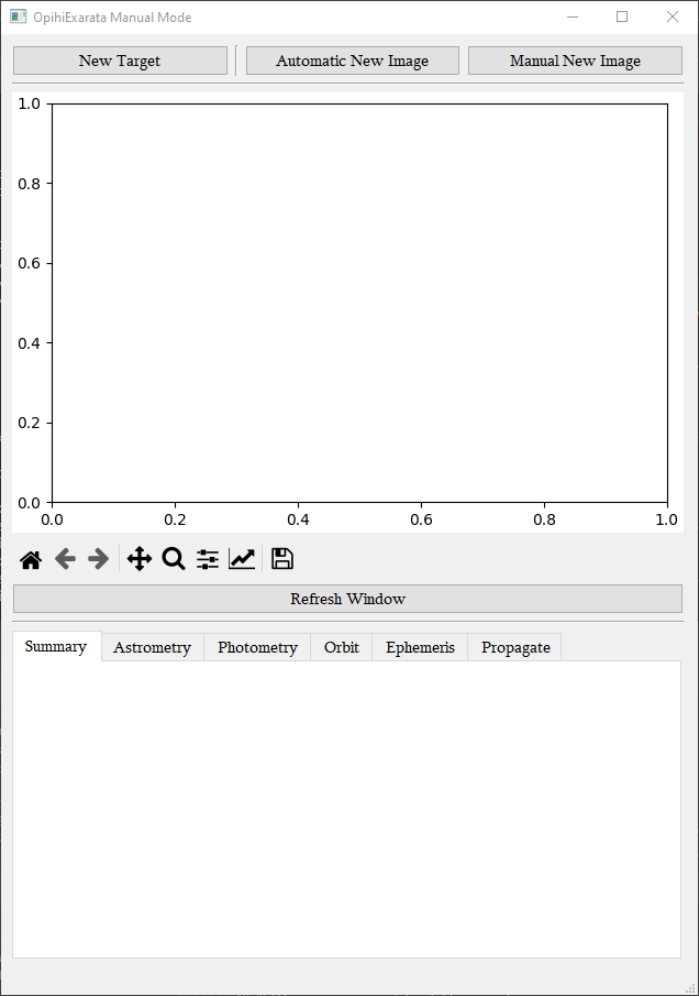
Fig. 2 The GUI of the manual mode of OpihiExarata. This is what you see when the interface is freshly loaded. Most of the text is filler text, they will change as the program is executed. Note that there are different tabs for the summary, astrometry, photometry, orbit, ephemeris, and propagation. Each of the sections covers their GUIs, this is just the general GUI.

The manual mode GUI contains a main data window and a few tabs compartmentalizing a lot of the functionality of OpihiExarata, see Fig. 2.

In the manual mode general GUI, you have three buttons which control file and target acquisition. The New Target button specifies that you desire to work on a new target (typically a new asteroid). The Manual New Image button opens a file dialog so that you can select a new Opihi image FITS file to load into OpihiExarata. The Automatic New Image button pulls the most recent FITS image from the same directory as the last image specified manually.

There is also a data viewer. Relevant information from the solutions will be plotted here along with the image data. There is a navigation bar for manipulating the image, including zooming, panning, saving, and configuring other options. This functionality makes use of matplotlib, see Interactive navigation (outdated) or Interactive figures for more information.

There is also a Refresh Window button to redraw the image in the viewer and to also refresh the information in the tabs. This should not be needed too much as the program should automatically refresh itself if there is new information.

Supplementary information is provided in the summary tab. This includes information about the path of the file, the filename, and methods to save the file.

A Send Target to TCS button allows for the user to send the target location (after astrometry has been executed) to the telescope operator and the telescope control software. Non-sidereal rates are sent as well if they were calculated via

Procedure

Fig. 3 A flowchart summary of the procedure of the manual mode. It includes the actions of the user along with the program’s flow afterwards.

We describe the procedure for utilizing the asteroid view-finding (manual) mode of OpihiExarata. See Fig. 11 for a flowchart summary of this procedure.

Start and Open GUI

You will want to open the OpihiExarata manual mode GUI, typically via the command-line interface with:

opihiexarata manual --config=config.yaml --secret=secrets.yaml

Please replace the configuration file names with the correct path to your configuration and secrets file; see Configuration for more information.

Specify New Target Name

The OpihiExarata manual mode software groups sequential images as belonging to a set of observations of a single target. In order to tell the software what target/asteroid you are observing you need to provide its name.

Use the New Target button, it will open a small prompt for you to enter the name of the asteroid/target you are observing. From this point on, all images loaded (either manually or automatically fetched) will be assumed to be of the target you provided (until you change it by clicking the button again).

Note

If you are observing an asteroid, this target name should also be the name of the asteroid. The software will attempt to use this name to obtain historical observations from the Minor Planet Center.

Take and Image

The first step in processing data is to take an image using the camera controller.

Note

It is highly suggested that you take two images if this is the first image you are taking of a given specified asteroid. This allows you to have a reference image which makes asteroid finding much easier. You process the first image normally (using the second image as the reference image) then process the second image (using the first image as the reference image). It does not matter which is the reference image for more images taken. (See Find Asteroid Location.)

Find Asteroid Location

You will need to find and specify the location of the asteroid in the image. It is beyond the scope of this software and procedure to implement this automatically. (If you are not observing asteroids, you may skip this step and just click Submit in the Target Selector GUI.)

Use the Target Selector GUI to find the asteroid pixel location.

Target Selector GUI

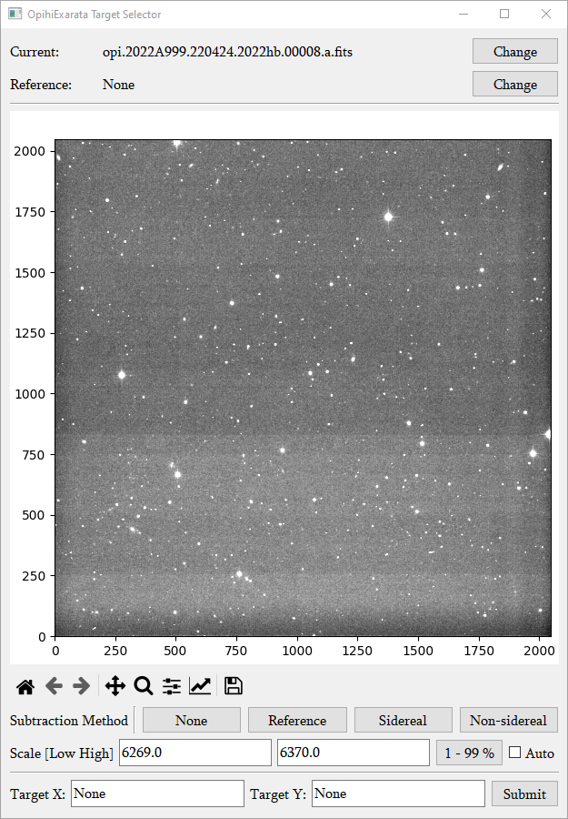
Fig. 4 The GUI for finding the pixel location of a target in the image. The targets are typically asteroids.

The target selector GUI allows you to select a specific target (generally an asteroid) location in an image, see Fig. 4.

The current file which you are determining the location of a target in is given by Current:. The reference image (if provided) used to compare against is given by Reference:. Both of these files can be changed using their respective Change buttons; a file dialog will be opened so you can specify the new FITS files.

There is a data viewer similar to the one specified in Graphical User Interface. However, in addition, if you drag a box (left click and hold, drag, then release) without any tool selected in toolbar, the software will search within the drawn (blue) box and extract the brightest object within the box. It will mark this target with a red triangle. It will assume that this is the desired target and update the Target X and Target Y fields with its pixel coordinates.

Note

This box drawing method finds the brightest object in the current image. It ignores the subtractive comparison method and its result as such comparisons do not affect the actual current image.

You can compare your current image file \(C\) with your reference image \(R\) file in two subtractive ways using the two labeled buttons under Subtraction Method. (There are also buttons for simply viewing the images.) Therefore, the two (plus two) ways of viewing the data are:

• None, \(C-0`\): The current image is not compared with the reference image.

• Reference, \(R-0\): The reference image is shown rather than the current image.

• Sidereal, \(C-R\): The two images are subtracted assuming the IRTF is doing sidereal tracking. Because of this assumption, no shifting is done.

• Non-sidereal, \(C-T_v(R)\): The two images are subtracted assuming the IRTF is doing non-sidereal tracking. Because of this assumption, the images are shifted based on the non-sidereal rates of the current image and the time between the two images.

The displayed image’s color bar scale can be modified manually by entering values into the boxes accompanying Scale [Low High], the left and right being the lower and higher bounds of the color bar respectively as indicated. The scale can also be automatically set so that the lower bound is the 1 percentile and the higher bound is the 99 percentile by clicking the 1 - 99 % button. If the Auto checkbox is enabled, this autoscaling is done whenever a new operation is done the image (i.e. using the tools in the toolbar, changing the comparison method, among others).

Select your target, either from the box method or by manually entering the coordinates in the Target X and Target Y boxes, and click Submit. The location of your target will be recorded.

Compute Astrometric Solution

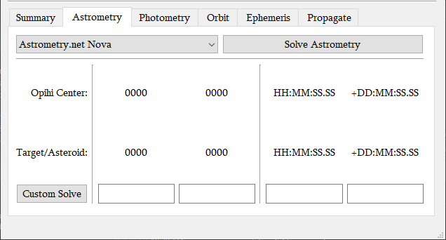
Fig. 5 The astrometry GUI tab for customizing and executing astrometric solutions. This is the default view before any values have been calculated.

The astrometric solution of the image is next to be solved. The pattern of stars within the image is compared with known patterns in astrometric star databases to derive the WCS astrometric solution of the image. See Fig. 5 for the interface for astrometric solutions.

To solve for the astrometric solution of the image, you will need to select the desired astrometric engine from the drop down menu then click on the Solve Astrometry button to solve. (See Services and Engines for more information on the available engines.)

The pixel location (X,Y) of the center of the image, given by Opihi Center, and the specified target, given by Target/Asteroid, is provided with or without an astrometric solution. When the astrometric solution is provided, the right ascension and declination of these will also be provided.

Custom pixel coordinate (X,Y) can be provided in the boxes to be translated to the sky coordinates that they correspond to. Alternatively, if sky coordinates are provided (in sexagesimal form, RA hours and DEC degrees, delimitated by colons), the pixel coordinates of the sky coordinates can also be determined; the pixel coordinate boxes must be empty as the solving gives preference to pixel to on-sky solving. Enter in either pixel or sky coordinates as described and click the Custom Solve button to convert it to the other. The button does nothing without a valid astrometric solution.

Compute Photometric Solution

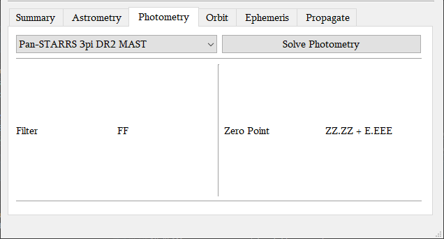
Fig. 6 The photometry GUI tab for customizing and executing photometric solutions. This is the default view before any values have been calculated.

The photometric solution of the image is next to be solved. The brightness of the stars in the image is compared to known filter magnitudes from a photometric database to derive a photometric calibration solution. See Fig. 6 for the interface for photometric solutions.

This is an optional step and is not related to asteroid finding in of itself. This operation can be skipped entirely if a photometric solution is not necessary.

To solve for the photometric solution of the image, you will need to select the desired photometric engine from the drop down menu then click on the Solve Photometry button to solve. (See Services and Engines for more information on the available engines.)

The filter that the image was taken in is noted by Filter, this is determined by the FITS file header.

Once a photometric solution has been solved, the corresponding filter zero point magnitude (and its error) of the image is provided by Zero Point.

Note

Execution of the photometric solution requires a completed astrometric solution from Compute Astrometric Solution.

Asteroid On-Sky Position

The asteroid pixel location is derived from the procedure in Target Selector GUI and the corresponding on-sky location is derived from the procedure in Compute Astrometric Solution.

Historical Observations

The software will attempt to use the target/asteroid name provided in Specify New Target Name to obtain the set of historical observations from the Minor Planet Center.

Recently taken images will also be considered part of the set of historical observations.

Asteroid Observation Record

The combination of both Historical Observations and Asteroid On-Sky Position makes up the sum total of the asteroid observation record. Using this asteroid observation record, the future path of the asteroid on the sky can be determined to eventually allow for the proper acquisition.

There are two different procedures for determining the future track of the asteroid:

• Propagating the on-sky motion of the asteroid into the future.

• Solving for the orbital elements and deriving an ephemeris.

Both options are sufficient but we recommend Asteroid Position Propagation.

Asteroid Position Propagation

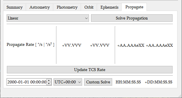
Fig. 7 The propagation GUI tab for customizing and executing propagation solutions. This is the default view before any values have been calculated.

Propagating the on-sky motion of the asteroid is done by taking the observational record from Asteroid Observation Record and propagating only the most recent observations forward in time. See Fig. 7 for the interface for propagation solutions.

To solve for the propagation solution from the observations, you will need to select the desired propagation engine from the drop down menu then click on the Solve Propagation button to solve. (See Services and Engines for more information on the available engines.)

If a propagation solution is done, the on-sky rates will be provided under Propagate Rate [ “/s | “/s²]. Both the first order (velocity) and second order (acceleration) on-sky rates in RA and DEC are given in arcseconds per second or arcseconds per second squared. The RA is given on the right and DEC on the left within the first or second order pairs. These rates may be sent to the TCS to update its non-sidereal rates vai the Update TCS Rate button after they are derived.

You may also provide a custom date and time, in the provided dialog box (using (ISO-8601 like formatting). You can specify the timezone that the provided date and time corresponds to using the dropdown menu. When you click Custom Solve, the displayed RA and DEC coordinates are the estimated sky coordinates for the asteroid at the provided input time.

Note

Execution of the propagation solution requires a completed astrometric solution from Compute Astrometric Solution.

Orbital Elements

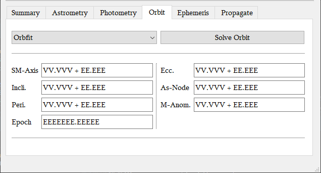
Fig. 8 The orbit GUI tab for customizing and executing orbital solutions. This is the default view before any values have been calculated.

Provided a list of historical observations, we can solve for the Keplerian orbital elements using preliminary orbit determination for osculating elements. See Fig. 8 for the interface for orbital solutions.

To solve for the orbital solution from the observations, you will need to select the desired orbit engine from the drop down menu then click on the Solve Orbit button to solve. (See Services and Engines for more information on the available engines.)

The six Keplerian orbital elements (plus the epoch) are provided after the orbital solution is solved. They are:

• SM-Axis: The semi-major axis of the orbit, this is in AU.

• Ecc.: The eccentricity of the orbit, this is unit-less.

• Incli.: The inclination of the orbit, in degrees.

• As-Node: The longitude of the ascending node, in degrees.

• Peri.: The argument of perihelion, in degrees.

• M-Anom.: The mean anomaly, in degrees.

• Epoch: The epoch of these of these osculating orbital elements, in Julian days.

If the Engine provided is Custom, then you are trying to provide a custom orbit. You provide your Keplerian orbital parameters in the boxes. You may also specify the error in these elements by providing another number delimitated from the first by a letter. (Note, scientific notation is not supported, especially E-notation based entries.) After you provide your orbital parameters, you can click Solve Orbit to solve for your orbital solution.

Note

Execution of the orbital solution requires a completed astrometric solution from Compute Astrometric Solution.

Ephemeris

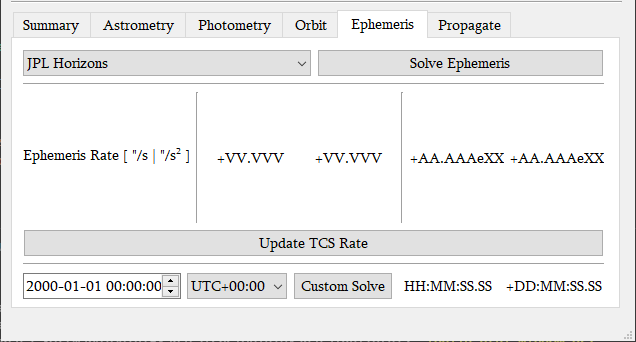
Fig. 9 The ephemeris GUI tab for customizing and executing ephemeris solutions. This is the default view before any values have been calculated.

The orbital elements derived in Orbital Elements can then be used to derive an ephemeris of an asteroid. See Fig. 9 for the interface for ephemeris solutions.

To solve for the ephemeris solution from the orbital elements, you will need to select the desired ephemeris engine from the drop down menu then click on the Solve Ephemeris button to solve. (See Services and Engines for more information on the available engines.)

If an ephemeris solution is done, the on-sky rates will be provided under Ephemeris Rate [ “/s | “/s²]. Both the first order (velocity) and second order (acceleration) on-sky rates in RA and DEC are given in arcseconds per second, or arcseconds per second squared. The RA is given on the right and DEC on the left within the first or second order pairs. These rates may be sent to the TCS to update its non-sidereal rates vai the Update TCS Rate button after they are derived.

You may also provide a custom date and time, in the provided dialog box (using ISO-8601 like formatting). You can specify the timezone that the provided date and time corresponds to using the dropdown menu. When you click Custom Solve, the displayed RA and DEC coordinates are the estimated sky coordinates for the asteroid at the provided input time.

Note

Execution of the ephemeris solution requires a completed orbital solution from Orbital Elements which itself depends on a completed astrometric solution from Compute Astrometric Solution.

Asteroid On-Sky Future Track

Regardless of which method you use to derive the future track of the asteroid (either from Asteroid Position Propagation or from Orbital Elements and Ephemeris), the future position of the asteroid and the on-sky rates are determined (see the respective sections for details).

Telescope Control Software: Update

The new asteroid on-sky future track (position and on-sky rates) derived from Asteroid On-Sky Future Track can be sent to the telescope control software to slew the telescope to the correct location of the asteroid.